AED Hallucinations - The Decoder Knows Too
In the previous articles, we established two things: the encoder of our AED model builds a near-perfect linear representation of speech vs non-speech from the very first transformer layer, and - crucially - this representation is causally upstream of the decoder. Steering encoder activations along the probe direction suppresses approximately 50% of hallucinations on non-speech audio, without measurably degrading transcription of real speech. Case A is confirmed: the model knows it is looking at non-speech; it simply fails to act on that knowledge.
This raises a natural follow-on question. When the decoder generates a hallucinated transcript - token by token, producing “Oh,” or “Thank you.” from ambient noise - does it build an internal representation of what it is doing? Does it, at the point of generation, “know” that it is hallucinating?
This is a distinct question from the encoder probe. The encoder is processing audio; we are asking whether the acoustic features it builds distinguish the two classes. Here, we are asking about the decoder’s state during generation - whether the hidden representations it constructs while producing output differ between hallucination and real transcription. The answer would tell us whether the failure to suppress hallucinations is isolated to the encoder-decoder interface, or whether it runs all the way through to the output stage.
Method
The method is identical in structure to the encoder probe, applied to the decoder layers. We register forward hooks on each decoder transformer layer during beam search. At each generation step, the new token’s hidden state is captured - with key-value caching enabled, each step processes exactly one new token, so the hook fires once per step and records a (hidden_dim,) vector. These are mean-pooled over the generated sequence to give one vector per example per layer.
The two classes are:
- Hallucination (
y = 0): non-speech audio where the model produced non-empty output - Normal (
y = 1): speech audio where the model produced a transcript
A logistic regression is trained per decoder layer, and 5-fold cross-validation gives unbiased accuracy estimates.
One subtlety: for non-speech audio, many segments produce no output at all - silence segments that the model correctly transcribes as silent. These contribute nothing to the hallucination class, since there is no decoder activation to probe. The collection therefore only retains examples where the model actually generated output, ensuring we are probing the decoder’s state during active hallucination rather than measuring the (trivially separable) difference between “generated something” and “generated nothing”.
Held-out evaluation
The collection loop tracks how many entries were scanned before the training set was filled. All entries beyond that scan boundary are held out and form a clean test set, guaranteed to have never been processed during training. This avoids any risk of leakage from examples that were scanned but discarded (e.g. non-hallucinating non-speech segments). The eval loop runs on this fully disjoint slice.
Results
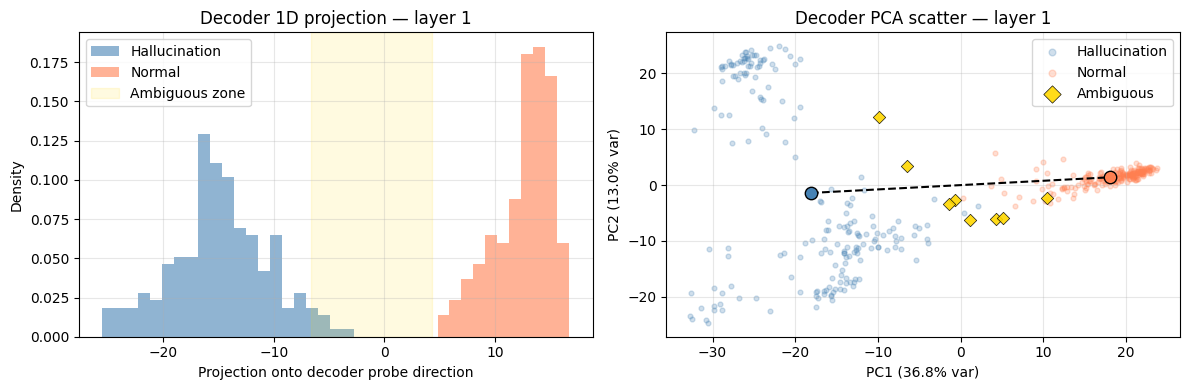
The decoder also separates
One important difference from the encoder probe is the choice of training data. The encoder probe used pure silence segments - acoustically unambiguous non-speech - against dense, fluent speech. The decoder probe here uses a harder, more realistic setting: the non-speech class consists of sparse speech segments - real audio containing speech interrupted by long pauses, background noise, and extended non-speech passages. These are exactly the segments most likely to cause hallucinations in production, and they represent the worst case for linear separability. The goal is to establish whether the separation holds even when the acoustic boundary between speech and non-speech is genuinely ambiguous.
The curve rises monotonically with depth, reaching above 0.97 towards the final layer. Unlike the encoder where separation is essentially complete from the very first layer, the decoder sharpens progressively - the signal is present early but becomes more linearly decodable as cross-attention information is integrated across the full stack.
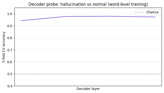
The 1D projection at the best layer shows essentially complete separation, with a gap of 7.6 pooled standard deviations between the two class centres.
Held-out evaluation: 99% recall, 99% precision
The fitted probe is evaluated on the held-out test set as a runtime hallucination detector: run the model, collect decoder activations, classify without looking at the transcript output.
| Correct | Errors | Rate | |
|---|---|---|---|
| Non-speech hallucinations | 458 detected | 5 missed | recall 0.99 |
| Speech transcriptions | 793 passed | 6 false positives | precision 0.99 |
Of 463 hallucinating segments in the test set, 458 are correctly identified. Of 799 normal speech segments, 793 are correctly cleared. 11 cases in total appear as errors. The correctly detected hallucinations are characteristic of the failure mode: short, affirmative-sounding fragments produced from ambient silence - “Oh,”, “Hold on.”, “Thank you.”, “I’m gonna go with it.”, “Jesus.” - consistent with what was observed in the encoder steering experiments.
The errors are labelling noise
On audio inspection of all 11 apparent errors, every single one is a labelling error in the evaluation dataset - not a probe failure.
The 5 false negatives - hallucinations the probe missed - are non-speech segments that actually contain speech. While the model transcribes them correctly, the probe correctly classifies them as normal transcription, i.e. the label is wrong.
| Type | Model output | Why it’s a label error |
|---|---|---|
| FN | Hey, Laluquet. Laluquet. | Audible speech in a segment marked as silence |
| FN | Michael. | Audible name in a silence segment |
| FN | it, man. | Audible speech fragment in a silence segment |
| FN | like my family. | Audible speech in a silence segment |
| FN | Сколько вообще инвестиций… | Audible Russian speech - correctly transcribed, mislabelled as non-speech |
Five of the 6 false positives are mirror-image labelling errors: segments labelled as speach that, on listening, contain no intelligible speech content. Despite the probe classifying these as hallucinations, they are actually correct.
| Type | Model output | Why it’s a label error |
|---|---|---|
| FP | Okay. | Segment contains no intelligible speech; output is a hallucination |
| FP | Um, | Borderline segment; no clear speech content |
| FP | Session. | Segment contains no intelligible speech |
| FP | Oh. | Segment contains no intelligible speech |
| FP | And, | Very short segment (~1.2s); no intelligible speech content |
The sixth is a genuine probe error. The segment contains difficult-to-follow speech, the model produces a transcript that does not match what is being said, and the probe flags it as a hallucination - which it is not. This is a real failure: the probe misclassifies a poor-quality transcription as a hallucination.
| Type | Model output | Assessment |
|---|---|---|
| FP | I got him here. | Genuine probe error - speech present, transcript incorrect but not a hallucination |
10 of the 11 apparent errors are labelling noise in the evaluation dataset. One is a genuine probe failure.
Where the signal lives: cross-attention, not generation
Evaluating the probe per individual token - rather than on the mean-pooled sequence - reveals something unexpected. For a subset of cases, every individual generated token is classified as normal by the probe, yet the overall mean-pooled activation is classified as a hallucination. Since the probe is a linear classifier, this can only happen if the mean is being pulled across the decision boundary by an activation not included in the per-token breakdown.
The culprit is the prefix activation: the decoder’s hidden state captured when it processes the initial [BOS, LANG] tokens before generating anything. This is the moment of the decoder’s first cross-attention over the encoder output - before a single transcript token exists. It is excluded from the per-token breakdown, but included in the mean.
A concrete example. A speech segment produces the output “And,” and the overall probe fires (false positive). The per-token breakdown looks like this:
| Position | Token | Probe classification |
|---|---|---|
| 0 | [prefix] |
hallucination |
| 1 | And | normal |
| 2 | , | normal |
The prefix is the only hallucination-classified position. Everything the decoder generated looks normal; only its initial state - set before generation begins, purely through cross-attention to the encoder - looks like a hallucination.
This tells us something about the nature of the undelrying mechanism here. The prefix activation is the decoder’s first and only opportunity to read the encoder output without any autoregressive context. Its state at that point is entirely determined by what the encoder produced - which is itself a near-perfect linear representation of speech vs non-speech. For non-speech audio, the encoder output sits deep in the non-speech cluster; the decoder’s initial cross-attention read of that output puts it in the hallucination region before any token is generated. For speech audio, the encoder output sits in the speech cluster; the initial cross-attention puts the decoder in the normal zone, and it stays there.
The implication is that the halucination signal in the decoder is encoded primarily in the initial cross-attention state, not in the autoregressive generation. The decoder does not become progressively more “aware” that it is hallucinating as it generates tokens - it knows from the very first step, before producing a single word, because it has already read the encoder’s non-speech representation. The tokens that follow are then generated from a starting point that already carries the hallucination signal in its mean-pooled representation. The cross-attention is the mechanism and everything else is downstream.
Ablation: ruling out sequence-length confounds
Two potential confounds are worth addressing. The first is transcript length: hallucinated transcripts are short (typically one to three words) while normal transcripts are long. The second is audio duration: silence segments used for the hallucination class may be systematically shorter than the speech segments, meaning the decoder’s cross-attention attends over a shorter encoder sequence - and the probe might be learning this length difference rather than anything about acoustic content.
Two ablations are run:
- Transcript position: the probe is retrained using only the first word of each segment. At position 0, both classes are in the same place in the sequence; any remaining separation must come from cross-attention content.
- Audio duration: the probe is retrained using only segments whose natural duration falls within the overlap window between the two classes. Segments are used whole - not trimmed - to avoid the risk of cutting a speech segment down to a silent passage.
| Full probe | First-word | Duration-matched | |
|---|---|---|---|
| First layer | 0.942 | 0.927 | 0.894 |
| Last layer | 0.973 | 0.972 | 0.969 |
The first-word probe barely moves - consistent with the positional confound being structurally implausible in any case, since the primary signal carrier is the prefix activation, computed before any token exists. Duration matching causes a ~5 percentage point drop in the first layer, suggesting the earliest decoder layer is somewhat sensitive to encoder sequence length; by the final layer the gap has closed to under half a point as deeper cross-attention integration takes over. Both ablations confirm that the separation is primarily grounded in acoustic content.
Interpretation
The decoder builds its own independent representation distinguishing hallucination from normal transcription, to essentially the same accuracy as the encoder probe. The model does not merely process non-speech audio differently in the encoder - it also generates tokens differently when hallucinating. Its internal state during hallucination generation is linearly distinguishable from its state during real transcription, consistently, across all four decoder layers, with no learning beyond a logistic regression.
This means the model has redundant, multilayerd knowledge that it is hallucinating. We show that the encoder has it from layer 0 and that the decoder builds it from generation step 1, but neither representation surfaces in the output.
The suppression achieved by encoder-level steering works not because it introduces new information into the system, but because it amplifies a signal the model already possesses. The decoder probe shows the complementary side of this: the decoder would, if it had a way to act on its own internal state, be capable of flagging its output as hallucinated.
The information required to suppress hallucinations is present in the model twice over - once at the input stage, once at the output stage. What is absent is not a training signal - non-speech and sparse-speech data were included in training, and the model does produce silence in the typical case. What is absent is a training objective that explicitly rewards the model for routing through the latent representation the probe identifies. The coupling between its internal knowledge that it is hallucinating and the decision to output EOS is loose enough to fail at the margin.
A secondary finding worth noting: the decoder probe is precise enough to function as an approximate label auditor. Applied to a labelled dataset, it surfaces samples where the label and the audio content disagree. This is not its intended use, but it suggests that interpretability tools applied at the output-generation stage can detect annotation noise that are otherwise challenging to identify.