Image Generation with GANs
Introduction
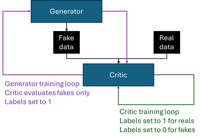
Generative Adversarial Networks (or GANs) are a really compelling framework for producing generative content. In the GAN framework, two networks are pitted against one another: one producing samples imitating the target content, while the other attempts to discriminate between the generated and real examples. An analogy that is often invoked is that of an art forger and an art critic, where the forger creates fake paintings which the critic then tries to identify. The two networks are often referred to as the ‘critic’ (or the ‘discriminator’) and the ‘generator’.
In this post I will explore the simplest case, where the critic is trained using binary cross entropy loss, which technically makes the term discriminator more appropriate (more on that later), but I will refer to it as a critic throughout.

The two networks compete (hence ‘adversarial’ in the name) and use one another to improve. The loss function of the critic is essentially how well it is able to assign probabilities of an image being real to the examples it is presented with, while the generator receives feedback on the probabilities the critic ascribed to its creations. Notably, the generator is never exposed to the actual distribution of the content it is trying to mimic (i.e. it does not learn directly from the data) — all feedback it receives is mediated by the critic, in the form of probabilities of the generated images being real.
The generator attempts to maximise the expression corresponding to the critic’s loss. To pose this as a minimisation problem for the generator, generated images are passed through the critic network alongside inverted labels (essentially just a vector of 1s). If the critic scores the image as real (outputs a probability close to 1), this results in a small difference between the score and the supplied label, and consequently a small generator loss. Note that this forward pass through the critic is not used in the training of the critic — this would be actively counter-productive, as the supplied labels are incorrect; it is just a trick to produce a minimisation problem for the generator.
Vanishing gradient
One issue with GANs is that both networks must learn at similar rates. If one network improves at a systematically faster rate, it will overpower its counterpart.
If, say, the critic is much more adept at recognising fakes than the generator is at creating realistic output, all the generator will receive as feedback is a sequence of 0s — it will know its output is poor, but it won’t know how to act on it. In practice, it is indeed the case that the critic tends to outgun the generator; this is largely because the critic’s job is easier — all it has to do is recognise whether an input is likely to have come from a distribution other than the target set. In contrast, the generator has to map out and learn the target space, generate a wide variety of examples from that space, while ensuring they all remain valid.
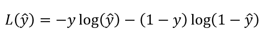
One network becoming vastly better than its counterpart leads to an example of the ‘vanishing gradient problem’. When the critic becomes very confident (and correct) in its predictions, those predictions are probabilities produced by a sigmoid activation in the critic’s final layer. Sigmoid’s gradient approaches zero as the input approaches negative infinity (which it does as the critic outputs increasingly confident 0s). This propensity to output 0s and 1s is a feature of the critic’s architecture and the binary cross entropy loss function in particular — it is also why, in this implementation, the critic is sometimes referred to as a discriminator, since it tends to evolve to near-binary outputs.
This can be addressed by altering the loss function; intuitively, we would like a continuum of scores not bounded between 0 and 1, so that gradient information continues flowing to the generator even if what it produces is highly mismatched with the target distribution. I will delve into this more in the next post.
Mode collapse
Another issue which stems from the vanishing gradient is ‘mode collapse’. The generator works by accepting a random noise vector as input into the generation process, providing a unique seed for each item to ensure diversity. The dimensionality of the noise vector should be sufficient to parametrise the latent space of the distribution being mimicked; we have no control over how the generator ascribes its specific dimensions to the individual dimensions of the input vector, but we need to give it a sufficient number of independent parameters to make sense of that space.
The content we are trying to mimic will most likely have a number of different ‘modes’ — regions of the latent space that result in a particular ‘type’ or ‘flavour’ of output. For example, if training the generator to produce realistic handwritten digits, a particular combination of values in the input vector will produce a 9, and small perturbations will also produce 9s. As we shift the parameters more and more, we gradually traverse the latent space until we move out of the range of values for 9 and start generating something more like an 8.
The way the model utilises the dimensions of the input vector evolves as the model trains. So a fixed input vector which started out by producing a 3 could, over time, start corresponding to a 9. This is exactly what you can see in the animation below — observe the evolution over 200 epochs of the digit in the bottom-right cell, which starts off as a 3 but gradually joins up into something more akin to a 9. Other cells also flicker between different digits.

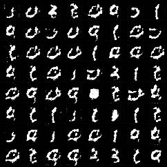
The problems start when the generator struggles to generate realistic outputs but somehow manages to produce a particular digit — say, a 0 — that fools the critic slightly better than other digits. The generator may then alter its weights so that 0s are produced more frequently. This works in the short term (which is the only term gradient descent cares about), but over time, as the critic catches up and starts outputting confidently low probabilities, the generator’s gambit proves disastrous: with gradient now vanished, it cannot find its way out of the position it has evolved into, where it outputs 0s regardless of the initial input. All modes have collapsed into just one, and there’s no way back.
An example of this kind of collapse is shown below. The animation shows the evolution of the generator’s output for a fixed set of noise inputs; the still on the right shows the final image after ~500 epochs. While the digits start off with quite a bit of diversity across the population, the final state shows that after a while some digits — in this case zeros and ones — are significantly over-represented.
In the next post, I will explore approaches to dealing with both the vanishing gradient problem and mode collapse, by investigating how the training rate of the two component models can be kept in alignment.